Fast.ai Chapter 3: MNIST Digit classifier, SGD, Optimiser and Sigmoid Function

Welcome to the chapter 3 of the fast.ai course. In the previous chapter, we created an image classifier and hosted it on the HuggingFace spaces. In this chapter, We will look deep inside the process behind all this and what are the steps involved in training an image classifier? We are going the cover the following things on this chapter -

• Creating a Handwritten Digit Classifier (using Pixel similarity)

• What is Stochastic Gradient Descent (SGD) ?

• How to calculate Gradients?

• How to decide the learning rate(lr) and minimise the Loss.

• Sigmoid Function and Why do we need it?

• Creating an Optimiser.

• Adding Non-Linearity to our models and why is it important.

• Putting it all together (Digit classifier using ML)

Building a digit classifier using pixel similarity

The digit classifier was one of the first ML applications that pushed the field forward. We're going to use the MNIST database, which has almost 60,000 images (28×28) in the training set and about 10,000 images of the same size in the test set.

Instead of training a model, we'll first use a pixel-similarity approach as our baseline. Imagine you have thousands of transparent sheets, with a single handwritten digit on each one. If you stack all the sheets with the same digit on top of each other, you'll see a rough outline of that digit. The outline will be solid in some places and faded in others.

To classify a new image, you'd pick a test digit from the test dataset and compare it to each of these stacked figures. The one that it most closely resembles is your answer.

Instead of using all the images, let's demonstrate this with just two digits: 3 and 7. We'll take all the images of 3s, convert them to a NumPy array, and divide them by 255. Since we have grayscale images, each of the 784 pixels (28×28) will be represented by a number between 0 (black) and 255 (white). Dividing by 255 will make the value of each pixel between 0 and 1. After that, we'll stack them in an array and take their mean to find the average value for each pixel.

threes = [np.array(Image.open(o).convert("L"))/255 for o in all_threes]
sevens = [np.array(Image.open(o).convert("L"))/255 for o in all_sevens]

threes_stack = np.stack(threes, axis=0)
sevens_stack = np.stack(sevens, axis=0)

mean3 = threes_stack.mean(axis=0)
mean7 = sevens_stack.mean(axis=0)
    

After taking the mean, we can pick a test image and find the difference between the pixels of the test image and the pixels of mean3 and mean7. The answer is the one with the lower difference.

img = np.array(Image.open(i).convert("L"))/255

diff3 = mean3 - img
diff7 = mean7 - img

if np.abs(diff3).sum() < np.abs(diff7).sum():
    print("This is a 3")
else:
    print("This is a 7")

You can find the notebook containing complete code here.

A special note about Numpy Broadcasting

If the code like np.array() / 255 feels a bit confusing, you might want to quickly look into Numpy broadcasting. This is a powerful feature that lets you perform operations between an array and a single number (a scalar), or even between arrays that don't have the same exact shape. For instance, when we divide an image array by 255, Numpy automatically knows to divide every single number in the array by 255. It's like it's stretching that single number to match the size of the whole array, making your code cleaner and more efficient.

Stochastic Gradient Descent (SGD)

Imagine you're trying to find the lowest point in a vast, hilly landscape.

Gradient Descent (GD) is like having a perfect, detailed topographical map of the entire landscape. You study the map carefully, identify the precise steepest downhill path, and take one big, deliberate step. You repeat this process, re-analysing the entire map for each step. This method is incredibly accurate, but because you have to analyse the whole map every time, it's very slow, especially on a huge landscape. This can lead to you getting stuck in a local valley (a "local minimum") because your careful analysis will only show you downhill paths within that valley, not the potential for an even deeper valley elsewhere.

Stochastic Gradient Descent (SGD) is different. You don't have a map of the whole landscape. Instead, you're standing in a thick fog. All you can do is feel the ground right under your feet and take a quick step in that downhill direction. Your steps are fast and a bit unpredictable because you're only reacting to a tiny part of the landscape at a time. This "stumbling" or "jittering" motion helps you avoid getting trapped in small, shallow valleys. You might not take the most perfect step each time, but over many quick steps, you'll generally make your way toward a very low point in the landscape.

What to Do When SGD Gets Stuck

Even with its "stumbling" nature, SGD can still get trapped in a deep but not-the-deepest valley. To solve this, we give our fog-walker some smarter tools, which are advanced optimisation techniques:

• Momentum: Think of this as giving our walker a slight shove in the direction they were already going. This push helps them keep moving, even if the ground temporarily flattens out or slopes slightly uphill. This "inertia" can propel them right out of a shallow valley and toward a deeper one.

• Adaptive Learning Rates (like Adam): This is like giving our walker a smart brain. When they're on a very steep slope, they take big, confident steps. As the ground starts to level out and they approach a minimum, they automatically take smaller, more cautious steps to avoid overshooting the lowest point.

By using these techniques and a lot of other, we get the best of both worlds: the speed of SGD with the added intelligence to avoid getting stuck in suboptimal spots.

We follow the below seven steps to train the model -

1. Initialise the weights

2. Predict which digit it is.

3. Calculate loss based on the prediction

4. Find the gradient for each weight.

5. Update the weights based on the gradient values.

6. Go back to step 2 and repeat the same process.

7. Iterate until you decide to stop the training process.

How to calculate Gradients

If you remember calculus, we can figure out the rate of change of any function by finding its derivative. We use the chain rule to find the derivative of a complex function.

The good news is we don't need to calculate anything manually. PyTorch does an amazing job of calculating gradients automatically if we set requires_grad=True. We just need to call the .backward() function on the loss, and then we can get the gradients for any variable.

def model(x, weights, bias):
    return x@weights+bias

def loss(preds, targets):
    predictions = preds.sigmoid()
    return torch.where(targets==1, 1-predictions, predictions).mean()
    

preds = model(train_x, weights, bias)
l = loss(preds, train_y)
l.backward()

After calling the function, PyTorch automatically populates the .grad property of the variables, and we can access it for both weights and bias. The great thing is that PyTorch keeps track of all the actions performed on a variable to reach the final loss and finds the gradient by taking care of the whole chain.

weight_grad = weights.grad
bias_grad = bias.grad

Learning rate and how to minimise loss

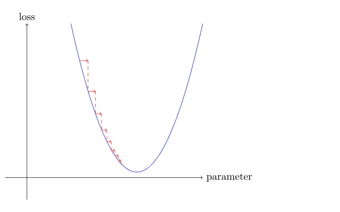
Once we have the gradients, we need to adjust our variables based on them. Learning rate decides the size of the step we take to update the variables (weights and bias). We should be cautious about setting it too low (it will take forever to make a significant change) or too high (the gradient will keep swinging from a high value to a low value and back again).

Once we have updated the variables, we should set the gradients back to zero. Otherwise, they will keep accumulating and won't update the variable correctly. The learning rate is a matter of trying a few values to find which one works best.

lr = 0.01
weights -= weights.grad * lr
bias -= bias.grad * lr
weights.grad.zero_()
bias.grad.zero_()

Sigmoid Function

When we predict values using the equation preds = x@w + b, the outputs can be anywhere on the real number line. But we need them to be between 0 and 1 to represent categories. The Sigmoid function does this by mapping every value to the range (0,1). It also has a smooth, continuous curve, which makes it easy to compute gradients.

def sigmoid(x): return 1/(1+torch.exp(-x))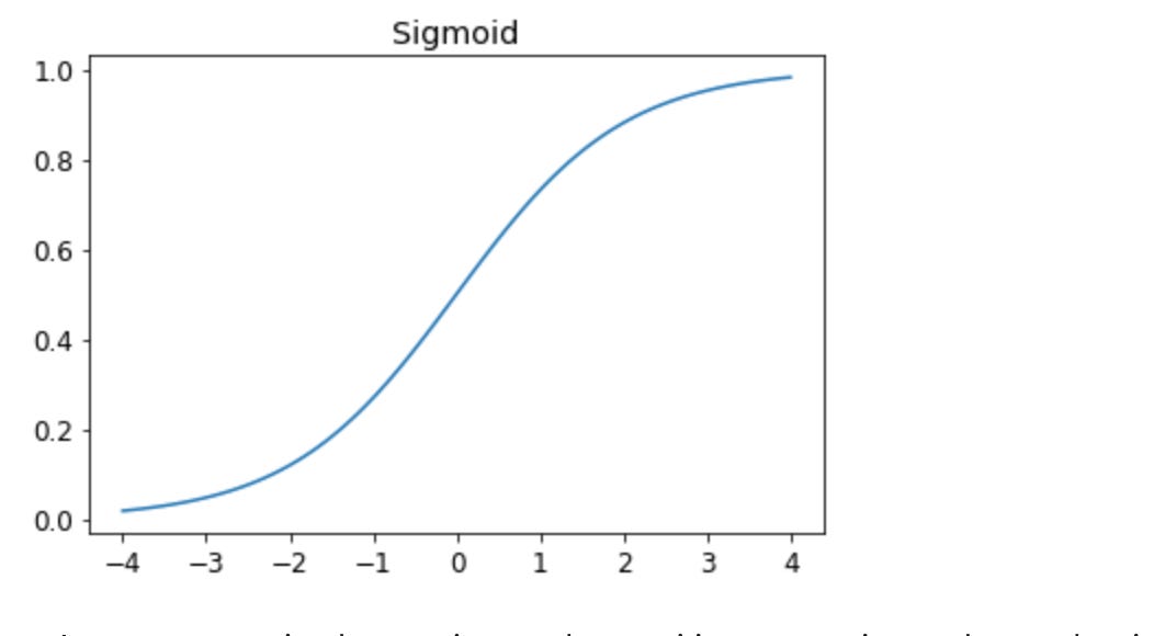

Creating an Optimiser

What we did by creating a linear function, finding loss and gradients, and then updating the variables (weights and bias), PyTorch provides us with classes to do all of these very efficiently. We can use torch.nn.linear, which does the same thing as initialising weights and bias and then what our linear function does. Using this information, we can create a basic optimizer.

class BasicOptim:
    def __init__(self,params,lr): 
        self.params = list(params)
        self.lr = lr

    def step(self, *args, **kwargs):
        for p in self.params: 
            p.data -= p.grad.data * self.lr

    def zero_grad(self, *args, **kwargs):
        for p in self.params: 
            p.grad = None

Note: Fast.ai provides a class (SGD) which does the same as BasicOptim.

Non-Linearity

We created a linear model (x@w +b is the equation for linear equation) in this tutorial and optimised it to categorise digits. But if we need to perform complex tasks, we need to introduce some complexity. We can do that by introducing non-linearity. But if we add a lot of linear functions, the result can still be represented by a single linear function.

To make it non-linear, we use a function called the Rectified Linear Unit (ReLU). It's a very simple function that replaces every negative number with zero. Now, if we add two linear functions (essentials lines) after passing them through ReLU, the result will be non-linear.

def ReLU(x):
    return np.maximum(0, x)

In 1990s, the computer scientist tried to use a single layer with ever increasing number of weights to get better results. The use of multiple layers with less weights did not gain any traction till 2000s. That’s when real shift in ML happened. Adding multiple layers even with less number of variables produced much better results than single layer with large number of variables.

Putting it all together (The ML Approach)

Let's build the digit classifier again, using everything we discussed. Let's assume we assign one variable for each pixel (called weights), which will be multiplied by the pixel values of the image. Then, we adjust our weights so they give a different result for each digit when multiplied. The better we are at adjusting these weights, the better our model will be at predicting.

In the very early days, the computer scientist used to set these weights manually which was a time consuming and quite difficult process. Now, we just set random weights and use gradient to find the best solution from there.

We will initialize the weights randomly with the same size as our images. Also, since many pixel values in our images are zero, if we only multiply them by weights, they won't contribute anything. So, we'll need something to add, which we call a bias. Let's initialize both weights and bias with requires_grad, because we'll need that for optimization.

# Let's define a matrix of same size as images with random weights
weights = torch.randn((28*28),1)).requires_grad_() 
bias = torch.randn(1)

Next, we need to multiply the weights by the image pixels and add the bias. One way to do this is element-wise multiplication and then summing them. Or, we can do matrix multiplication, which does the same thing.

# Both of these do the same 
y = (img*weights.T).sum() + bias
y_mat = img@weights.T+bias

Instead of multiplying one image at a time and looping through all the images—which takes a lot of time—we can stack all the images and multiply them at once using a PyTorch tensor. Using a tensor is fast because it's a single operation, and we can run it on a GPU in parallel for multiple images. We stacked all the 3s and 7s and put them in one variable (train_x). After that, we made a dependent variable (train_y) with 1s and 0s as the output.

threes = torch.stack([torch.tensor(np.array(Image.open(o).convert("L"))) for o in all_threes])
sevens = torch.stack([torch.tensor(np.array(Image.open(o).convert("L"))) for o in all_sevens])

train_x = torch.cat([threes, sevens]).view(-1, 28*28).float()
train_y = torch.tensor([0]*len(threes) + [1]*len(sevens)).unsqueeze(1)

Then we use our linear and loss functions defined above to optimize the weights and bias. For training our model, we're going to put our images in batches using the DataLoader class.

from torch.utils.data import DataLoader
dls = list(zip(train_x, train_y))
dl = DataLoader(dls, batch_size=256)

Then we iterate over the dataloader and train our model. We define an epoch as going over all the images once.

def epoch(lr, weights, bias):
    for xb, yb in dl:
        preds = model(xb, weights, bias)
        l = loss(preds, yb)
        l.backward()
        with torch.no_grad():
            weights -= weights.grad * lr
            bias -= bias.grad * lr
            weights.grad.zero_()
            bias.grad.zero_()

Then, we train our model for some epochs until we find optimized values.

for i in range(30):
    epoch(.1, weights, bias)
    print(i, validate_epoch(weights, bias))

That's it. We have created a linear model from scratch and used it to classify digits. You can access the complete notebook here.

My Experiments and what broke down

First of all, there is only one notebook for this lecture, which shows the pixel similarity approach. There is no specific notebook for the ML approach. You have to create it yourself by reading the chapter and using the code given there. So, I made one for the ML approach, which you can access above.

While training this model, I used the whole training set of images before updating the weights instead of doing it after every batch using dataloaders. I put in a lot of effort and still couldn't get more than 57% accuracy, which is not better than a random guess and much worse than our pixel similarity approach. After I used the dataloaders and updated weights using batches, the accuracy swiftly went up to 96%.

It's about making multiple small adjustments rather than one big adjustment at a time, which keeps the gradients swaying.

Wrap up

Well that’s a wrap up for lesson 3.

• We started with a pixel similarity approach as a baseline and saw how simple comparisons can already give good results.

• Then we built a proper ML model step by step — introducing gradients, loss, learning rate, optimisers, and non-linearity.

• The biggest learning was the power of mini-batches. Updating weights in small steps gave us much better accuracy (~96%) compared to using the whole dataset at once (~57%).

• This chapter showed how simple building blocks come together to form a complete training loop.

Next, we’ll keep stacking these ideas and build stronger, more flexible models.

P.S. If you enjoyed this post, consider subscribing to my mailing list. I’ll be writing one blog for each chapter of the Fast.ai course, along with my experiments, as wells as on career advice and startups.

Don’t worry—I won’t spam you with cat memes… unless you’re into that 🐱. Just practical insights, resources, and maybe a joke or two to keep things fun.

If you found this post helpful, would you please consider re-stacking it and sharing it with other people?